Search

Friday, April 07, 2017

A comment on the DeLong et al 2005 nine-labs replication failure

Nieuwland et al replication attempts of DeLong at al. 2005

Note: Revised 8 April 2017 following comments from Nieuwland and others.

Recently, Nieuwland et al did an interesting series of replication attempts of the DeLong et al 2005 Nature Neuroscience paper. Nieuwland et al report a failure to replicate the original effect. This is just a quick note to suggest that it may be difficult to claim that this is a replication failure. I focus only on the article data.

First we load the Nieuwland et al data (available from https://osf.io/eyzaq).

articles <-read.delim("public_article_data.txt", quote="")
#head(articles)

Then make sure columns are correct data types, and get lab names, convert cloze to z-scores as Nieuwland et al did:

articles$item <-as.factor(articles$item)
articles$cloze <- as.numeric(as.character(articles$cloze))

labnames<-unique(articles$lab)

# Z-transform cloze and prestimulus interval
articles$zcloze <- scale(articles$cloze, center = TRUE, scale = TRUE)
articles$zprestim <- scale(articles$prestim, center = TRUE, scale = TRUE)

Then use lmer to compute estimates from each lab separately. I also fit ``maximal’’ models in Stan (HT: Barr et al 2013 ;) but nothing much changes so I use these varying slopes models without correlations:

library(lme4)
## Loading required package: Matrix
# models for article fit for each lab separately:
res<-matrix(rep(NA,9*2),ncol=2)
for(i in 1:9){
model <- lmer(base100 ~ zcloze + ( 1| subject) +
                (zcloze|| item), 
              data = subset(articles,lab==labnames[i]),
                control=lmerControl(
                  optCtrl=list(maxfun=1e5)))
res[i,]<-summary(model)$coefficients[2,1:2]
}

Next, we fit a random-effects meta-analysis using the nine-labs replications.

Random effects meta-analysis:

The model specification was as follows.

Assume that:

  1. \(y_i\) is the observed effect in microvolts in the \(i\)-th study with \(i=1\dots n\);
  2. \(\theta\) is the true (unknown) effect, to be estimated by the model;
  3. \(\sigma_{i}^2\) is the true variance of the sampling distribution; each \(\sigma_i\) is estimated from the standard error available from the study \(i\);
  4. The variance parameter \(\tau^2\) represents between-study variance.

We can construct a random-effects meta-analysis model as follows:

\[\begin{equation} \begin{split} y_i \mid \theta_i,\sigma_i^2 \sim & N(\theta_i, \sigma_i^2) \quad i=1,\dots, n\\ \theta_i\mid \theta,\tau^2 \sim & N(\theta, \tau^2), \\ \theta \sim & N(0,10^2),\\ \tau \sim & N(0,10^2)T(0,) \hbox{(truncated normal)} \\ \end{split} \end{equation}\]

The priors shown above are just examples. Other priors can be used and are probably more suitable in this case. I use Gelman et al 2014’s non-centralized parameterization in any case in the Stan code below because of the sparse data we have here.

## Stan meta-analysis:
library(rstan)
## Loading required package: ggplot2
## Loading required package: StanHeaders
## rstan (Version 2.14.1, packaged: 2017-01-20 19:24:23 UTC, GitRev: 565115df4625)
## For execution on a local, multicore CPU with excess RAM we recommend calling
## rstan_options(auto_write = TRUE)
## options(mc.cores = parallel::detectCores())
rstan_options(auto_write = TRUE)
options(mc.cores = parallel::detectCores())

dat<-list(y=res[,1],n=length(res[,1]),s=res[,2])

## is this the DeLong et al mean and se? Could add it to meta-analysis if original data ever becomes available.
#dat$y<-c(dat$y,0.4507929)
#dat$s<-c(dat$s,.5)
#dat$n<-dat$n+1

fit <- stan(file='rema2.stan', data=dat,
            iter=2000, chains=4, seed=987654321,
            control = list(adapt_delta = 0.99))

paramnames<-c("mu","tau","theta")
print(fit,pars=paramnames,prob=c(0.025,0.975))
## Inference for Stan model: rema2.
## 4 chains, each with iter=2000; warmup=1000; thin=1; 
## post-warmup draws per chain=1000, total post-warmup draws=4000.
## 
##          mean se_mean   sd  2.5% 97.5% n_eff Rhat
## mu       0.11       0 0.07 -0.04  0.25  2153    1
## tau      0.11       0 0.08  0.00  0.31  1496    1
## theta[1] 0.11       0 0.10 -0.09  0.31  4000    1
## theta[2] 0.13       0 0.10 -0.08  0.36  4000    1
## theta[3] 0.10       0 0.11 -0.13  0.33  4000    1
## theta[4] 0.10       0 0.11 -0.13  0.30  4000    1
## theta[5] 0.03       0 0.11 -0.23  0.22  4000    1
## theta[6] 0.06       0 0.13 -0.25  0.27  4000    1
## theta[7] 0.14       0 0.11 -0.05  0.39  4000    1
## theta[8] 0.18       0 0.11  0.00  0.42  4000    1
## theta[9] 0.15       0 0.11 -0.04  0.40  4000    1
## 
## Samples were drawn using NUTS(diag_e) at Sat Apr  8 19:51:28 2017.
## For each parameter, n_eff is a crude measure of effective sample size,
## and Rhat is the potential scale reduction factor on split chains (at 
## convergence, Rhat=1).
params<-extract(fit,pars=paramnames)

Results

The interesting thing here is the posterior distribution of \(\mu\), the effect of cloze probability on the N400.

## posterior probability that mu is > 0:
mean(params$mu>0)
## [1] 0.9345
mean(params$mu)
## [1] 0.1084961
## lower and upper bounds of credible intervals:
lower<-quantile(params$mu,prob=0.025)
upper<-quantile(params$mu,prob=0.975)
SE<-(upper-lower)/4 ## approximate, assuming symmetry which seems reasonable here
hist(params$mu,main="Posterior distribution of effect \n Article",xlab="mu",freq=F)
abline(v=0)
arrows(x0=lower,y0=1,x1=upper,y1=1,angle=90,code=3)

Thus, even in the Nieuwland et al nine-labs data, the N400 amplitude decreases (becomes more positive) with increasing cloze probability. The posterior probability that the coefficient for cloze is greater than 0 is 94%. From this, one cannot really say that the Nieuwland et al studies are a failure to replicate the DeLong study.

The next step would be to compare the original DeLong et al data using the same analysis done above. But I was unable to get the original data up until now, so I’m posting my comment on my blog.

Prestimulus interval

Mante Nieuwland pointed out to me that the effect can be seen already in the prestimulus interval. Here is the evidence for that.

# models for article fit for each lab separately:
res<-matrix(rep(NA,9*2),ncol=2)
for(i in 1:9){
model <- lmer(prestim ~ zcloze + ( 1| subject) +
                (zcloze|| item), 
              data = subset(articles,lab==labnames[i]),
                control=lmerControl(
                  optCtrl=list(maxfun=1e5)))
res[i,]<-summary(model)$coefficients[2,1:2]
}

dat<-list(y=res[,1],n=length(res[,1]),s=res[,2])

## is this the DeLong et al mean and se? Could add it to meta-analysis if original data ever becomes available.
#dat$y<-c(dat$y,0.4507929)
#dat$s<-c(dat$s,.5)
#dat$n<-dat$n+1

fit <- stan(file='rema2.stan', data=dat,
            iter=2000, chains=4, seed=987654321,
            control = list(adapt_delta = 0.99))

paramnames<-c("mu","tau","theta")
print(fit,pars=paramnames,prob=c(0.025,0.975))
## Inference for Stan model: rema2.
## 4 chains, each with iter=2000; warmup=1000; thin=1; 
## post-warmup draws per chain=1000, total post-warmup draws=4000.
## 
##           mean se_mean   sd  2.5% 97.5% n_eff Rhat
## mu        0.07       0 0.07 -0.06  0.21  1497    1
## tau       0.12       0 0.08  0.01  0.30   897    1
## theta[1]  0.18       0 0.11  0.00  0.41  2632    1
## theta[2] -0.01       0 0.11 -0.26  0.17  2042    1
## theta[3]  0.11       0 0.11 -0.10  0.36  4000    1
## theta[4]  0.13       0 0.10 -0.04  0.34  4000    1
## theta[5]  0.03       0 0.09 -0.16  0.20  4000    1
## theta[6]  0.01       0 0.11 -0.23  0.20  4000    1
## theta[7]  0.03       0 0.10 -0.19  0.22  4000    1
## theta[8]  0.09       0 0.09 -0.08  0.28  4000    1
## theta[9]  0.11       0 0.09 -0.06  0.29  4000    1
## 
## Samples were drawn using NUTS(diag_e) at Sat Apr  8 19:51:33 2017.
## For each parameter, n_eff is a crude measure of effective sample size,
## and Rhat is the potential scale reduction factor on split chains (at 
## convergence, Rhat=1).
params<-extract(fit,pars=paramnames)

## posterior probability that mu is > 0:
mean(params$mu>0)
## [1] 0.88175
mean(params$mu)
## [1] 0.07359659
## lower and upper bounds of credible intervals:
lower<-quantile(params$mu,prob=0.025)
upper<-quantile(params$mu,prob=0.975)
SE<-(upper-lower)/4 ## approximate, assuming symmetry which seems reasonable here
hist(params$mu,main="Posterior distribution of effect \n Prestimulus interval",xlab="mu",freq=F)
abline(v=0)
arrows(x0=lower,y0=1,x1=upper,y1=1,angle=90,code=3)

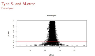
Retrospective power calculation

We now compute retrospective power and Type S/M errors:

## Gelman and Carlin function:
retrodesign <- function(A, s, alpha=.05, df=Inf, n.sims=10000){
  z <- qt(1-alpha/2, df)
  p.hi <- 1 - pt(z-A/s, df)
  p.lo <- pt(-z-A/s, df)
  power <- p.hi + p.lo
  typeS <- p.lo/power
  estimate <- A + s*rt(n.sims,df)
  significant <- abs(estimate) > s*z
  exaggeration <- mean(abs(estimate)[significant])/A
  return(list(power=power, typeS=typeS, exaggeration=exaggeration))
}

retrodesign(.11, SE)
## $power
##     97.5% 
## 0.3761173 
## 
## $typeS
##        97.5% 
## 0.0004168559 
## 
## $exaggeration
## [1] 1.616742

The bad news here is that if the meta-analysis posterior mean for the article is the true effect, then power is about 34%.

If we want about 80% power, we need to halve that SE:

retrodesign(.11, 0.072/2)
## $power
## [1] 0.8633715
## 
## $typeS
## [1] 3.063012e-07
## 
## $exaggeration
## [1] 1.079705

I think that implies that you need four times as many subjects than you had.

Acknowledgements

Thanks to Mante Nieuwland and Stephen Politzer-Ahles for patiently explaining a lot of details to me, and for sharing their data and code.

Appendix: Stan code

Here is the meta-analysis Stan code with the Gelman-style reparameterization. y_tilde is not used above, but yields posterior predictive values, and could be used profitably in future replication attempts.

data {
    int<lower=0> n; //number of studies
    real y[n]; // estimated effect
    real<lower=0> s[n]; // SEs of effect
}
parameters{
    real mu; //population mean
    real<lower=0> tau;  // between study variability    
    vector[n] eta; //study level errors
} 
transformed parameters {
    vector[n] theta;   // study effects
    theta = mu + tau*eta;
}
model {
eta ~ normal(0,1);
y ~ normal(theta,s);
}
generated quantities{
vector[n] y_tilde;
for(i in 1:n){
  y_tilde[i] = normal_rng(theta[i],s[i]); 
  }
}

Monday, March 27, 2017

Fitting Bayesian Linear Mixed Models for continuous and binary data using Stan: A quick tutorial

I want to give a quick tutorial on fitting Linear Mixed Models (hierarchical models) with a full variance-covariance matrix for random effects (what Barr et al 2013 call a maximal model) using Stan.

For a longer version of this tutorial, see: Sorensen, Hohenstein, Vasishth, 2016.

Prerequisites: You need to have R and preferably RStudio installed; RStudio is optional. You need to have rstan installed. See here. I am also assuming you have fit lmer models like these before:
lmer(log(rt) ~ 1+RCType+dist+int+(1+RCType+dist+int|subj) + (1+RCType+dist+int|item), dat)
If you don't know what the above code means, first read chapter 4 of my lecture notes.

The code and data format needed to fit LMMs in Stan

The data

I assume you have a 2x2 repeated measures design with some continuous measure like reading time (rt) data and want to do a main effects and interaction contrast coding. Let's say your main effects are RCType and dist, and the interaction is coded as int. All these contrast codings are $\pm 1$. If you don't know what contrast coding is, see these notes and read section 4.3 (although it's best to read the whole chapter). I am using an excerpt of an example data-set from Husain et al. 2014.
"subj" "item" "rt""RCType" "dist" "int"
1       14    438  -1        -1      1
1       16    531   1        -1     -1
1       15    422   1         1      1
1       18   1000  -1        -1      1 
...
Assume that these data are stored in R as a data-frame with name rDat.

The Stan code

Copy the following Stan code into a text file and save it as the file matrixModel.stan. For continuous data like reading times or EEG, you never need to touch this file again. You will only ever specify the design matrix X and the structure of the data. The rest is all taken care of.
data {
  int N;               //no trials
  int P;               //no fixefs
  int J;               //no subjects
  int n_u;             //no subj ranefs
  int K;               //no items
  int n_w;             //no item ranefs
  int subj[N]; //subject indicator
  int item[N]; //item indicator
  row_vector[P] X[N];           //fixef design matrix
  row_vector[n_u] Z_u[N];       //subj ranef design matrix
  row_vector[n_w] Z_w[N];       //item ranef design matrix
  vector[N] rt;                 //reading time
}

parameters {
  vector[P] beta;               //fixef coefs
  cholesky_factor_corr[n_u] L_u;  //cholesky factor of subj ranef corr matrix
  cholesky_factor_corr[n_w] L_w;  //cholesky factor of item ranef corr matrix
  vector[n_u] sigma_u; //subj ranef std
  vector[n_w] sigma_w; //item ranef std
  real sigma_e;        //residual std
  vector[n_u] z_u[J];           //spherical subj ranef
  vector[n_w] z_w[K];           //spherical item ranef
}

transformed parameters {
  vector[n_u] u[J];             //subj ranefs
  vector[n_w] w[K];             //item ranefs
  {
    matrix[n_u,n_u] Sigma_u;    //subj ranef cov matrix
    matrix[n_w,n_w] Sigma_w;    //item ranef cov matrix
    Sigma_u = diag_pre_multiply(sigma_u,L_u);
    Sigma_w = diag_pre_multiply(sigma_w,L_w);
    for(j in 1:J)
      u[j] = Sigma_u * z_u[j];
    for(k in 1:K)
      w[k] = Sigma_w * z_w[k];
  }
}

model {
  //priors
  beta ~ cauchy(0,2.5);
  sigma_e ~ cauchy(0,2.5);
  sigma_u ~ cauchy(0,2.5);
  sigma_w ~ cauchy(0,2.5);
  L_u ~ lkj_corr_cholesky(2.0);
  L_w ~ lkj_corr_cholesky(2.0);
  for (j in 1:J)
    z_u[j] ~ normal(0,1);
  for (k in 1:K)
    z_w[k] ~ normal(0,1);
  //likelihood
  for (i in 1:N)
    rt[i] ~ lognormal(X[i] * beta + Z_u[i] * u[subj[i]] + Z_w[i] * w[item[i]], sigma_e);
}

Define the design matrix

Since we want to test the main effects coded as the columns RCType, dist, and int, our design matrix will look like this:
# Make design matrix
X <- unname(model.matrix(~ 1 + RCType + dist + int, rDat))
attr(X, "assign") <- NULL

Prepare data for Stan

Stan expects the data in a list form, not as a data frame (unlike lmer). So we set it up as follows:
# Make Stan data
stanDat <- list(N = nrow(X),
P = ncol(X),
n_u = ncol(X),
n_w = ncol(X),
X = X,
Z_u = X,
Z_w = X,
J = nlevels(rDat$subj),
K = nlevels(rDat$item),
rt = rDat$rt,
subj = as.integer(rDat$subj),
item = as.integer(rDat$item))

Load library rstan and fit Stan model

library(rstan) 
rstan_options(auto_write = TRUE)
options(mc.cores = parallel::detectCores())

# Fit the model
matrixFit <- stan(file = "matrixModel.stan", data = stanDat,
iter = 2000, chains = 4)

Examine posteriors

print(matrixFit)
This print output is overly verbose. I wrote a simple function to get the essential information quickly.
stan_results<-function(m,params=paramnames){
  m_extr<-extract(m,pars=paramnames)
  par_names<-names(m_extr)
  means<-lapply(m_extr,mean)
  quantiles<-lapply(m_extr,
                    function(x)quantile(x,probs=c(0.025,0.975)))
  means<-data.frame(means)
  quants<-data.frame(quantiles)
  summry<-t(rbind(means,quants))
  colnames(summry)<-c("mean","lower","upper")
  summry
}
For example, if I want to see only the posteriors of the four beta parameters, I can write:
stan_results(matrixFit, params=c("beta[1]","beta[2]","beta[3]","beta[4]"))
For more details, such as interpreting the results and computing things like Bayes Factors, see Nicenboim and Vasishth 2016.

FAQ: What if I don't want to fit a lognormal?

In the Stan code above, I assume a lognormal function for the reading times:
 rt[i] ~ lognormal(X[i] * beta + Z_u[i] * u[subj[i]] + Z_w[i] * w[item[i]], sigma_e);
If this upsets you deeply and you want to use a normal distribution (and in fact, for EEG data this makes sense), go right ahead and change the lognormal to normal:
 rt[i] ~ normal(X[i] * beta + Z_u[i] * u[subj[i]] + Z_w[i] * w[item[i]], sigma_e);

FAQ: What if I my dependent measure is binary (0,1) responses?

Use this Stan code instead of the one shown above. Here, I assume that you have a column called response in the data, which has 0,1 values. These are the trial level binary responses.
data {
  int N;               //no trials
  int P;               //no fixefs
  int J;               //no subjects
  int n_u;             //no subj ranefs
  int K;               //no items
  int n_w;             //no item ranefs
  int subj[N]; //subject indicator
  int item[N]; //item indicator
  row_vector[P] X[N];           //fixef design matrix
  row_vector[n_u] Z_u[N];       //subj ranef design matrix
  row_vector[n_w] Z_w[N];       //item ranef design matrix
  int response[N];                 //response
}

parameters {
  vector[P] beta;               //fixef coefs
  cholesky_factor_corr[n_u] L_u;  //cholesky factor of subj ranef corr matrix
  cholesky_factor_corr[n_w] L_w;  //cholesky factor of item ranef corr matrix
  vector[n_u] sigma_u; //subj ranef std
  vector[n_w] sigma_w; //item ranef std
  vector[n_u] z_u[J];           //spherical subj ranef
  vector[n_w] z_w[K];           //spherical item ranef
}

transformed parameters {
  vector[n_u] u[J];             //subj ranefs
  vector[n_w] w[K];             //item ranefs
  {
    matrix[n_u,n_u] Sigma_u;    //subj ranef cov matrix
    matrix[n_w,n_w] Sigma_w;    //item ranef cov matrix
    Sigma_u = diag_pre_multiply(sigma_u,L_u);
    Sigma_w = diag_pre_multiply(sigma_w,L_w);
    for(j in 1:J)
      u[j] = Sigma_u * z_u[j];
    for(k in 1:K)
      w[k] = Sigma_w * z_w[k];
  }
}

model {
  //priors
  beta ~ cauchy(0,2.5);
  sigma_u ~ cauchy(0,2.5);
  sigma_w ~ cauchy(0,2.5);
  L_u ~ lkj_corr_cholesky(2.0);
  L_w ~ lkj_corr_cholesky(2.0);
  for (j in 1:J)
    z_u[j] ~ normal(0,1);
  for (k in 1:K)
    z_w[k] ~ normal(0,1);
  //likelihood
  for (i in 1:N)
    response[i] ~ bernoulli_logit(X[i] * beta + Z_u[i] * u[subj[i]] + Z_w[i] * w[item[i]]);
}

For reproducible example code

See here.

Tuesday, November 22, 2016

Statistics textbooks written by non-statisticians: Generally a Bad Idea

A methodologist from psychology called Russell Warne writes on twitter:


It is of course correct that you can usually increase power by increasing sample size. 

But a lot of the other stuff in this paragraph is wrong or misleading. If this is an introductory statistics textbook for psychologists, it will cause a lot of harm: a whole new generation of psychologists will emerge with an incorrect understanding of the frequentist point of view to inference. Here are some comments on his text:
  1. "When a study has low statistical power, it raises the possibility that any rejection of the null hypothesis is just a fluke, i.e., a Type I error": A fluke rejection of a null hypothesis, isn't that the definition of Type I error? So, low power raises the possibility that a rejection is a Type I error? There is so much wrong here. First of all, Type I error is associated with hypothetical replications of the experiment. It is a statement about the long run repetitions of the procedure, not about the specific experiment you did. You cannot talk of a particular result being a "Type I error" or not. Second, the above sentence says that if power is low, you could end up with an incorrect rejection; the implication is that if power is high, I am unlikely to end up with an incorrect rejection! What the author should have said is that when power is low, by definition the probability of correctly detecting the effect is low. Punkt. Furthermore, the much more alarming consequence of low power is Type S and M errors (see my next point below). I'm surprised that psychologists haven't picked this up yet.
  2.  When power is low, "...the study should most likely not have been able to reject the null hypothesis at all. So, when it does reject the null hypothesis, it does not seem like a reliable result": I think that one word that should be banned in psych* is "reliable", it gives people the illusion that they found out something that is true. It is never going to be the case that you can say with 100% certainty that you found out the truth. If reliable means "true, reflecting reality correctly", you will *never* know that you have a reliable result. The trouble with using words like reliable is when people read a sentence like the one above and then try to construct the meaning of the sentence by considering the converse situation, when power is high. The implication is that when power is high, the rejection of the result is "reliable". I have lost count of how many times I have heard psych* people telling me that a result is "reliable", implying that they found something that is true of nature. Even when power is high, you still have a Type I error of whatever your $\alpha$ is. So any individual result you get could be an incorrect rejection; it doesn't matter what you think the power is. A further important point is: how do you *know* what power you have? Due to Type S and M errors, you are most likely doing your calculation based on previous, underpowered studies. You are therefore going to be getting gross overestimates of power anyway. Power is a function, and typically, you will have a lot of uncertainty associated with your estimate of the plausible values of power under different assumptions (after all, you don't *know* what the true effect is, right? If you know already, why are you doing the study?).  Giving a student the false security of saying "oh, I have high power, so my result is reliable" is pretty irresponsible and is part of the reason why we keep messing up again and again and again.

Tuesday, August 02, 2016

Two papers, with code: Statistical Methods for Linguistic Research (Parts 1 and 2)

Here are two papers that may be useful for researchers in psychology, linguistics, and cognitive science:

Shravan Vasishth and Bruno Nicenboim. Statistical methods for linguistic research: Foundational Ideas - Part I. Language and Linguistics Compass, 2016. In Press. 
PDF: http://bit.ly/VasNicPart1
Code: http://bit.ly/VasNicPart1Code
Bruno Nicenboim and Shravan Vasishth. Statistical methods for linguistics research: Foundational Ideas - Part II. Language and Linguistics Compass, 2016. In Press.
PDF:  http://bit.ly/NicVasPart2
Code: http://bit.ly/NicVasPart2Code

Wednesday, April 27, 2016

A simple proof that the p-value distribution is uniform when the null hypothesis is true

[Scroll to graphic below if math doesn't render for you]

Thanks to Mark Andrews for correcting some crucial typos (I hope I got it right this time!).

Thanks also to Andrew Gelman for pointing out that the proof below holds only when the null hypothesis is a point null $H_0: \mu = 0$, and the dependent measure is continuous, such as reading time in milliseconds, or EEG responses.

Someone asked this question in my linear modeling class: why is it that the p-value has a uniform distribution when the null hypothesis is true? The proof is remarkably simple (and is called the probability integral transform).

First, notice that when a random variable Z comes from a $Uniform(0,1)$ distribution, then the probability that $Z$ is less than (or equal to) some value $z$ is exactly $z$: $P(Z\leq z)=z$.

Next, we prove the following proposition:

Proposition:
If a random variable $Z=F(T)$, then $Z \sim Uniform(0,1)$.

Note here that the p-value is a random variable, call it $Z$. The p-value is computed by calculating the probability of seeing a t-statistic or something more extreme under the null hypothesis. The t-statistic comes from a random variable $T$ that is a transformation of the random variable $\bar{X}$: $T=(\bar{X}-\mu)/(\sigma/\sqrt{n})$. This random variable T has a CDF $F$.

So, if we can prove the above proposition, we have shown that the p-value's distribution under the null hypothesis is $Uniform(0,1)$.

Proof:

Let $Z=F(T)$.

$P(Z\leq z) = P(F(T)\leq z) = P(F^{-1} F(T) \leq F^{-1}(z) )
= P(T \leq F^{-1} (z) )
= F(F^{-1}(z))= z$.

Since $P(Z\leq z)=z$, Z is uniformly distributed, that is, Uniform(0,1).

A screengrab in case the above doesn't render:


Sunday, January 17, 2016

Automating R exercises and exams using the exams package

It's a pain to design statistics exercises each semester, and because students from previous share old exercises with the new incoming students, it's hard to design simple exercises that students haven't already seen the answers to. On top of that, some students try to cheat during the exam by looking over the shoulder of their neighbors. Homework exercises almost always involve collaboration even if you prohibit it.

It turns out that you can automate the generation of fixed-format exercises (with different numerical answers being required each time). You can also randomly select questions from a question bank you create yourself. And you can even create a unique question paper for each student in an exam, to make cheating between neighbors essentially impossible (even if they copy the correct answer to question 2 from a neighbor, they end up answering the wrong question on their own paper).

All this magic is made possible by the exams package in R. The documentation is of course comprehensive and there is a journal article explaining everything:
Achim Zeileis, Nikolaus Umlauf, Friedrich Leisch (2014). Flexible Generation of E-Learning Exams in R: Moodle Quizzes, OLAT Assessments, and Beyond. Journal of Statistical Software 58(1), 1-36. URL http://www.jstatsoft.org/v58/i01/.
I also use this package to deliver auto-graded exercises to students over datacamp.com. See here for the course I teach, and here for the datacamp exercises.

Here is a quick example to get people started on designing their own customized, automated exams. In my example below, there are several files you need.

1. The template files for your exam (what your exam or homework sheet will look like), and the solutions file. I provide two example files: test.tex and solutiontest.tex

2. The exercises or exam questions themselves: I provide two as examples. The first file is called pnorm1.Rnw. It's an Sweave file, and it contains the code for generating a random problem and for generating its solution. The code should be self-explanatory. The second file is called sesamplesize1multiplechoice.Rnw and has a multiple choice question.

3.  The exam generating R code file: The code is commented and self-explanatory. It will generate the exercises, randomize the order of presentation (if there are two or more exercises), and generate a solutions file. The output will be a single or multiple exam papers (depending on how many versions you wanted generated), and the solutions file(s).  Notice the cool thing that even in my example, with only one question, the two versions of the exams have different numbers, so two people cannot collaborate and consult each other and just write down one answer.  Each student could in principle be given a unique set of exercises, although it would be a lot of work to grade it if you do it manually.

Here is the exam generating code:

Save from the gists given above (a) the test.tex and solutiontest.tex files, (b) the Rnw files containing the exercise (pnorm1.Rnw, and sesamplesize1multiplechoice.Rnw), and (c) the exam generating code (ExampleExamCode.R).  Put all of these into your working directory, say ExampleExam. Then run the R code, and be amazed.

If something is broken in my example, please let me know.
 
Shuffling questions: If you want to reorder the questions in each run of the R code, just change myexamlist to sample(myexamlist) in the call below that appears in the file ExampleExamCode.R:

sol <- exams(sample(myexamlist), n = num.versions, 
             dir = odir, template = c("test", "solutiontest"),
             nsamp=1,
             header = list(ID = getID, Date = Sys.Date()))


Wednesday, January 06, 2016

My MSc thesis: A meta-analysis of relative clause processing in Mandarin Chinese using bias modelling

Here is my MSc thesis, which was submitted to the University of Sheffield in September 2015. 

The pdf is here.

Title: A Meta-analysis of Relative Clause Processing in Mandarin Chinese using Bias Modelling

Abstract
The reading difficulty associated with Chinese relative clauses presents an important empirical problem for psycholinguistic research on sentence comprehension processes. Some studies show that object relatives are easier to process than subject relatives, while others show the opposite pattern. If Chinese has an object relative advantage, this has important implications for theories of reading comprehension.  In order to clarify the facts about Chinese, we carried out a Bayesian random-effects meta-analysis using 15 published studies; this analysis showed that the posterior probability of a subject relative advantage is approximately $0.77$ (mean $16$, 95% credible intervals $-29$ and $61$ ms). Because the studies had significant biases, it is possible that they may have confounded the results. Bias modelling is a potentially important tool in such situations because it uses expert opinion to incorporate the biases in the model. As a proof of concept, we first identified biases in five of the fifteen studies, and elicited priors on these using the SHELF framework. Then we fitted a random-effects meta-analysis, including priors on biases. This analysis showed a stronger posterior probability ($0.96$) of a subject relative advantage compared to the standard random-effects meta-analysis (mean $33$, credible intervals $-4$ and $71$).

Saturday, December 19, 2015

Best statistics-related comment ever from a reviewer

This is the most interesting comment I have ever received from CUNY conference reviewing. It nicely illustrates the state of our understanding of statistical theory in psycholinguistics:

"I had no idea how many subjects each study used. Were just one or two people
used? ... Generally, I wasn't given enough data to determine my confidence in the provided t-values (which depends on the degrees of freedom involved)."
 

Thursday, August 27, 2015

Five thirty-eight provides a brand new definition of the p-value

The Five-Thirty Eight blog provides a brand new definition of the p-value: 
http://fivethirtyeight.com/datalab/psychology-is-starting-to-deal-with-its-replication-problem/?ex_cid=538twitter

"A p-value is simply the probability of getting a result at least as extreme as the one you saw if your hypothesis is false."

I thought this blog was run by Nate Silver, a statistician?

Observed vs True Statistical Power, and the power inflation index

People (including me) routinely estimate statistical power for future studies using a pilot study's data or a previously published study's data (or perhaps using the predictions from a computational model, such as Engelmann et al 2015).

Indeed, the author of the Replicability Index has been using observed power to determine the replicability of journal articles. His observed power estimates are HUGE (in the range of 0.75) and seem totally implausible to me, given the fact that I can hardly ever replicate my studies.

This got me thinking: Gelman and Carlin have shown that when power is low, Type M error will be high. That is, the observed effects will tend to be highly exaggerated. The issue with Type M error is easy to visualize.

Suppose that a particular study has standard error 46, and sample size 37; this implies that standard deviation is $46\times \sqrt{37}= 279$. These are representative numbers from psycholinguistic studies. Suppose also that we know that the true effect (the absolute value, say on the millisecond scale for a reading study---thanks to Fred Hasselman) is D=15. Then, we can compute Type S and Type M errors for replications of this particular study by repeatedly sampling from the true distribution.

We can visualize the exaggerated effects under low power as follows (see below): On the x-axis you see the effect magnitudes, and on the y-axis is power. The red line is the power line of 0.20, which based on my own attempts at replicating my own studies (and mostly failing), I estimate to be an upper bound of the power of experiments in psycholinguistics (this is an upper bound, I think a more common value will be closer to 0.05). All those dots below the red line are exaggerated estimates in a low power situation, and if you were to use any of those points to estimate observed power, you would get a wildly optimistic power estimate which has no bearing with reality.


What does this fact about Type M error imply for Replicability Index's calculations? It implies that if power is in fact very low, and if journals are publishing larger-than-true effect sizes (and we know that they have an incentive to do so, because editors and reviewers mistakenly think that lower p-values, i.e., bigger absolute t-values, give stronger evidence for the specific alternative hypothesis of interest), then Replicability Index is possibly hugely overestimating power, and therefore hugely overestimating replicability of results.

I came up with the idea of framing this overestimation in terms of Type M error by defining something called a power inflation index. Here is how it works. For different "true" power levels, we repeatedly sample data, and compute observed power each time. Then, for each "true" power level, we can compute the ratio of the observed power to the true power in each case. The mean of this ratio is the power inflation index, and the 95% confidence interval around it gives us an indication (sorry Richard Morey! I know I am abusing the meaning of CI here and treating it like a credible interval!) of how badly we could overestimate power from a small sample study.

Here is the code for simulating and visualizing the power inflation index:


And here is the visualization:

What we see here is that if true power is as low as 0.05 (and we can never know that it is not since we never know the true effect size!), then using observed power can lead to gross overestimates by a factor of approximately 10! So, if Replicability Index reports an observed power of 0.75, what he might actually be looking at is an inflated estimate where true power is 0.08.

In summary, we can never know true power, and if we are estimating it using observed power conditional on true power being extremely low, we are likely to hugely overestimate power.

One way to test my claim is to actually try to replicate the studies that Replicability Index predicts has high replicability. My prediction is that his estimates will be wild overestimates and most studies will not replicate. 

Postscript

A further thing that worries me about Replicability Index is his sloppy definitions of statistical terms. Here is how he defines power:

"Power is defined as the long-run probability of obtaining significant results in a series of exact replication studies. For example, 50% power means that a set of 100 studies is expected to produce 50 significant results and 50 non-significant results."

[Thanks to Karthik Durvasula for correcting my statement below!]
By not defining power of a test of a null hypothesis $H_0: \mu=k$, as the probability of rejecting the null hypothesis (as a function of different alternative $\mu$ such that $\mu\neq k$) when it is false, what this definition literally means is that if I sample from any distribution, including one where $\mu=0$, the probability of obtaining a significant result under repeated sampling is the power. Which of course is completely false.

Post-Post Script

Replicability Index points out in a tweet that his post-hoc power estimation corrects for inflation. But post-hoc power corrected for inflation requires knowledge of the true power, which is what we are trying to get at in the first place. How do you deflate "observed" power when you don't know what the true power is? Maybe I am missing something.