The original paper and the main claims
The data are from this paper:
Fedorenko, E., Gibson, E., & Rohde, D. (2006). The nature of working memory capacity in sentence comprehension: Evidence against domain-specific working memory resources. Journal of Memory and Language, 54(4), 541-553.
Ev was kind enough to give me the data; many thanks to her for this.
Design
The study is a self-paced reading experiment, with a 2x2x2 design, the examples are as follows:
- Factor: One noun in memory set or three nouns
easy: Joel
hard: Joel-Greg-Andy
- Factor: Noun type, either proper name or occupation
name: Joel-Greg-Andy
occ: poet-cartoonist-voter
- Factor: Relative clause type (two versions, between subjects but within items—we ignore this detail in this blog post):
- Subject-extracted, version 1: The physician | who consulted the cardiologist | checked the files | in the office.
- Subject-extracted, version 2: The cardiologist | who consulted the physician | checked the files | in the office.
- Object-extracted, version 1: The physician | who the cardiologist consulted | checked the files | in the office.
- Object-extracted, version 2: The cardiologist | who the physician consulted | checked the files | in the office.
As hinted above, this design is not exactly 2x2x2; there is also a within items manipulation of relative clause version. That detail was ignored in the published analysis, so we ignore it here as well.
The main claims in the paper
The main claim of the paper is laid out in the abstract above, but I repeat it below:
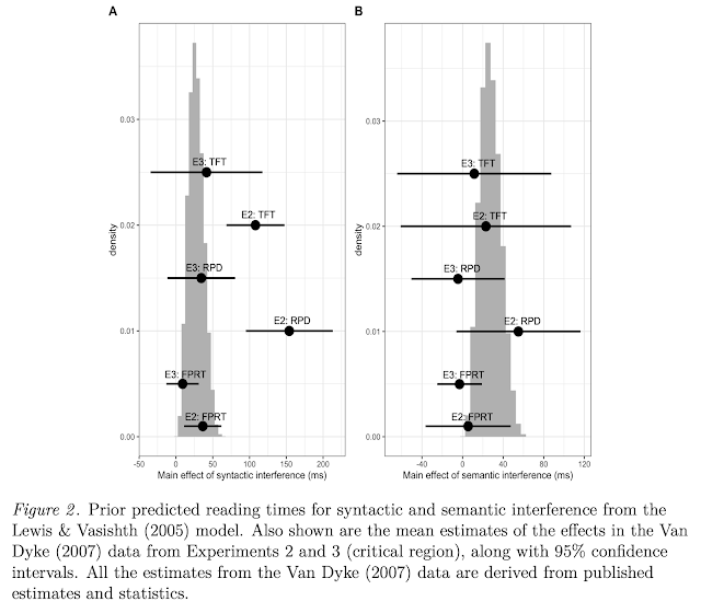
“A significant on-line interaction was found between syntactic complexity and similarity between the memory-nouns and the sentence-nouns in the three memory-nouns conditions, such that the similarity between the memory-nouns and the sentence-nouns affected the more complex object-extracted relative clauses to a greater extent than the less complex subject-extracted relative clauses.”
The General Discussion explains this further. I highlight the important parts.
“The most interesting result presented here is an interaction between syntactic complexity and the memory- noun/sentence-noun similarity during the critical region of the linguistic materials in the hard-load (three memory-nouns) conditions: people processed object-extracted relative clauses more slowly when they had to maintain a set of nouns that were similar to the nouns in the sentence than when they had to maintain a set of nouns that were dissimilar from the nouns in the sentence; in contrast, for the less complex subject-extracted relative clauses, there was no reading time difference between the similar and dissimilar memory load conditions. In the easy-load (one memory-noun) conditions, no interaction between syntactic complexity and memory-noun/sentence-noun similarity was observed. These results provide evidence against the hypothesis whereby there is a pool of domain-specific verbal working memory resources for sentence comprehension, contra Caplan and Waters (1999). Specifically, the results reported here extend the off-line results reported by Gordon et al. (2002) who—using a similar dual-task paradigm—provided evidence of an interaction between syntactic complexity and memory-noun/sentence-noun similarity in response-accuracies to questions about the content of the sentences. Although there was also a suggestion of an on-line reading time interaction in Gordon et al.’s experiment, this effect did not reach significance. The effect of memory-noun type in subject-extracted conditions was 12.7 ms per word (50.8ms over the four-word relative clause region), and the effect of memory-noun type in object-extracted conditions was 40.1 ms (160.4 ms over the four-word relative clause region). (Thanks to Bill Levine for providing these means). In the hard-load conditions of our experiment, the effect of memory-noun type in subject-extracted conditions over the four-word relative clause region is 12 ms in raw RTs (18 ms in residual RTs), and the effect of memory- noun type in object-extracted conditions is 324 ms in raw RTs (388 ms in residual RTs). This difference in effect sizes of memory-noun type between Gordon et al.’s and our experiment is plausibly responsible for the interaction observed in the current experiment, and the lack of such an interaction in Gordon et al.’s study. The current results therefore demonstrate that Gordon et al.’s results extend to on-line processing.”
The statistical evidence in the paper for the claim
Table 3 in the paper (last line) reports the critical interaction claimed for the hard-load conditions (I added the p-values, which were not provided in the table):
“Synt x noun type [hard load]: F1(1,43)=6.58, p=0.014;F2(1,31)=6.79, p=0.014”.
There is also a minF’ provided: \(minF'(1,72)=3.34, p=0.07\). I also checked the minF’ using the standard formula from a classic paper by Herb Clark:
Clark, H. H. (1973). The language-as-fixed-effect fallacy: A critique of language statistics in psychological research. Journal of Verbal Learning and Verbal Behavior, 12(4), 335-359.
[Aside: The journal “Journal of Verbal Learning and Verbal Behavior” is now called Journal of Memory and Language.]
Here is the minF’ function:
minf <- function(f1,f2,n1,n2){
fprime <- (f1*f2)/(f1+f2)
n <- round(((f1+f2)*(f1+f2))/(((f1*f1)/n2)+((f2*f2)/n1)))
pval<-pf(fprime,1,n,lower.tail=FALSE)
return(paste("minF(1,",n,")=",round(fprime,digits=2),"p-value=",round(pval,2),"crit=",round(qf(.95,1,n))))
}
And here is the p-value for the minF’ calculation:
minf(6.58,6.79,43,31)
## [1] "minF(1, 72 )= 3.34 p-value= 0.07 crit= 4"
The first thing to notice here is that even the published claim (about an RC type-noun type interaction in the hard load condition) is not statistically significant. I have heard through the grapevine that JML allows the authors to consider an effect as statistically significant even if the MinF’ is not significant. Apparently the reason is that the MinF’ calculation is considered to be conservative. But if they are going to ignore it, why the JML wants people to report a MinF’ is a mystery to me.
Declaring a non-significant result to be significant is a very common situation in the Journal of Memory and Language, and other journals. Some other JML papers I know of that report a non-significant minF’ as their main finding in the paper, but still act as if they have significance are:
Dillon et al 2013: “For total times this analysis revealed a three-way interaction that was significant by participants and marginal by items (\(F_1(1,39)=8.0,...,p=<0.01; F_1(1,47)=4.0,...,p=<0.055; minF'(1,81)=2,66,p=0.11\))”.
Van Dyke and McElree 2006: “The interaction of LoadxInterference was significant, both by subjects and by items. … minF’(1,90)=2.35, p = 0.13.”
Incidentally, neither of the main claims in these two studies replicated (which is not the same thing as saying that their claims are false—we don’t know whether they are false or true):
- Replication attempt of Dillon et al 2013: Lena A. Jäger, Daniela Mertzen, Julie A. Van Dyke, and Shravan Vasishth. Interference patterns in subject-verb agreement and reflexives revisited: A large-sample study. Journal of Memory and Language, 111, 2020.
- Replication attempt of Van Dyke et al 2006: Daniela Mertzen, Anna Laurinavichyute, Brian W. Dillon, Ralf Engbert, and Shravan Vasishth. Is there cross-linguistic evidence for proactive cue-based retrieval interference in sentence comprehension? Eye-tracking data from English, German and Russian. submitted, 2021
The second paper was rejected by JML, by the way.
Data analysis of the Fedorenko et al 2006 study
## Download and install library from here:
## https://github.com/vasishth/lingpsych
library(lingpsych)
data("df_fedorenko06")
head(df_fedorenko06)
##    rctype nountype load item subj region   RT
## 2     obj     name hard   16    1      2 4454
## 6    subj     name hard    4    1      2 5718
## 10   subj     name easy   10    1      2 2137
## 14   subj     name hard   20    1      2  903
## 18   subj     name hard   12    1      2 1837
## 22   subj      occ hard   19    1      2 1128
As explained above, we have a 2x2x2 design: rctype [obj,subj] x nountype [name, occupation] x load [hard,easy]. Region 2 is the critical region, the entire relative clause, and RT is the reading time for this region. Subject and item columns are self-explanatory.
We notice immediately that something is wrong in this data frame. Compare subject 1 vs the other subjects:
## something is wrong here:
xtabs(~subj+item,df_fedorenko06)
##     item
## subj 1 2 3 4 5 6 7 8 9 10 11 12 13 14 15 16 17 18 19 20 21 22 23 24 25 26 27 28
##   1  2 2 2 2 2 2 2 2 2  2  2  2  2  2  2  2  2  2  2  2  2  2  2  2  2  2  2  2
##   2  1 1 1 1 1 1 1 1 1  1  1  1  1  1  1  1  1  1  1  1  1  1  1  1  1  1  1  1
##   3  1 1 1 1 1 1 1 1 1  1  1  1  1  1  1  1  1  1  1  1  1  1  1  1  1  1  1  1
##   4  1 1 1 1 1 1 1 1 1  1  1  1  1  1  1  1  1  1  1  1  1  1  1  1  1  1  1  1
##   5  1 1 1 1 1 1 1 1 1  1  1  1  1  1  1  1  1  1  1  1  1  1  1  1  1  1  1  1
##   6  1 1 1 1 1 1 1 1 1  1  1  1  1  1  1  1  1  1  1  1  1  1  1  1  1  1  1  1
##   7  1 1 1 1 1 1 1 1 1  1  1  1  1  1  1  1  1  1  1  1  1  1  1  1  1  1  1  1
##   8  1 1 1 1 1 1 1 1 1  1  1  1  1  1  1  1  1  1  1  1  1  1  1  1  1  1  1  1
##   9  1 1 1 1 1 1 1 1 1  1  1  1  1  1  1  1  1  1  1  1  1  1  1  1  1  1  1  1
##   11 1 1 1 1 1 1 1 1 1  1  1  1  1  1  1  1  1  1  1  1  1  1  1  1  1  1  1  1
##   12 1 1 1 1 1 1 1 1 1  1  1  1  1  1  1  1  1  1  1  1  1  1  1  1  1  1  1  1
##   13 1 1 1 1 1 1 1 1 1  1  1  1  1  1  1  1  1  1  1  1  1  1  1  1  1  1  1  1
##   14 1 1 1 1 1 1 1 1 1  1  1  1  1  1  1  1  1  1  1  1  1  1  1  1  1  1  1  1
##   15 1 1 1 1 1 1 1 1 1  1  1  1  1  1  1  1  1  1  1  1  1  1  1  1  1  1  1  1
##   16 1 1 1 1 1 1 1 1 1  1  1  1  1  1  1  1  1  1  1  1  1  1  1  1  1  1  1  1
##   17 1 1 1 1 1 1 1 1 1  1  1  1  1  1  1  1  1  1  1  1  1  1  1  1  1  1  1  1
##   18 1 1 1 1 1 1 1 1 1  1  1  1  1  1  1  1  1  1  1  1  1  1  1  1  1  1  1  1
##   19 1 1 1 1 1 1 1 1 1  1  1  1  1  1  1  1  1  1  1  1  1  1  1  1  1  1  1  1
##   20 1 1 1 1 1 1 1 1 1  1  1  1  1  1  1  1  1  1  1  1  1  1  1  1  1  1  1  1
##   21 1 1 1 1 1 1 1 1 1  1  1  1  1  1  1  1  1  1  1  1  1  1  1  1  1  1  1  1
##   22 1 1 1 1 1 1 1 1 1  1  1  1  1  1  1  1  1  1  1  1  1  1  1  1  1  1  1  1
##   23 1 1 1 1 1 1 1 1 1  1  1  1  1  1  1  1  1  1  1  1  1  1  1  1  1  1  1  1
##   24 1 1 1 1 1 1 1 1 1  1  1  1  1  1  1  1  1  1  1  1  1  1  1  1  1  1  1  1
##   25 1 1 1 1 1 1 1 1 1  1  1  1  1  1  1  1  1  1  1  1  1  1  1  1  1  1  1  1
##   26 1 1 1 1 1 1 1 1 1  1  1  1  1  1  1  1  1  1  1  1  1  1  1  1  1  1  1  1
##   28 1 1 1 1 1 1 1 1 1  1  1  1  1  1  1  1  1  1  1  1  1  1  1  1  1  1  1  1
##   29 1 1 1 1 1 1 1 1 1  1  1  1  1  1  1  1  1  1  1  1  1  1  1  1  1  1  1  1
##   30 1 1 1 1 1 1 1 1 1  1  1  1  1  1  1  1  1  1  1  1  1  1  1  1  1  1  1  1
##   31 1 1 1 1 1 1 1 1 1  1  1  1  1  1  1  1  1  1  1  1  1  1  1  1  1  1  1  1
##   32 1 1 1 1 1 1 1 1 1  1  1  1  1  1  1  1  1  1  1  1  1  1  1  1  1  1  1  1
##   33 1 1 1 1 1 1 1 1 1  1  1  1  1  1  1  1  1  1  1  1  1  1  1  1  1  1  1  1
##   34 1 1 1 1 1 1 1 1 1  1  1  1  1  1  1  1  1  1  1  1  1  1  1  1  1  1  1  1
##   35 1 1 1 1 1 1 1 1 1  1  1  1  1  1  1  1  1  1  1  1  1  1  1  1  1  1  1  1
##   36 1 1 1 1 1 1 1 1 1  1  1  1  1  1  1  1  1  1  1  1  1  1  1  1  1  1  1  1
##   37 1 1 1 1 1 1 1 1 1  1  1  1  1  1  1  1  1  1  1  1  1  1  1  1  1  1  1  1
##   38 1 1 1 1 1 1 1 1 1  1  1  1  1  1  1  1  1  1  1  1  1  1  1  1  1  1  1  1
##   39 1 1 1 1 1 1 1 1 1  1  1  1  1  1  1  1  1  1  1  1  1  1  1  1  1  1  1  1
##   40 1 1 1 1 1 1 1 1 1  1  1  1  1  1  1  1  1  1  1  1  1  1  1  1  1  1  1  1
##   41 1 1 1 1 1 1 1 1 1  1  1  1  1  1  1  1  1  1  1  1  1  1  1  1  1  1  1  1
##   42 1 1 1 1 1 1 1 1 1  1  1  1  1  1  1  1  1  1  1  1  1  1  1  1  1  1  1  1
##   43 1 1 1 1 1 1 1 1 1  1  1  1  1  1  1  1  1  1  1  1  1  1  1  1  1  1  1  1
##   44 1 1 1 1 1 1 1 1 1  1  1  1  1  1  1  1  1  1  1  1  1  1  1  1  1  1  1  1
##   46 1 1 1 1 1 1 1 1 1  1  1  1  1  1  1  1  1  1  1  1  1  1  1  1  1  1  1  1
##   47 1 1 1 1 1 1 1 1 1  1  1  1  1  1  1  1  1  1  1  1  1  1  1  1  1  1  1  1
##     item
## subj 29 30 31 32
##   1   2  2  2  2
##   2   1  1  1  1
##   3   1  1  1  1
##   4   1  1  1  1
##   5   1  1  1  1
##   6   1  1  1  1
##   7   1  1  1  1
##   8   1  1  1  1
##   9   1  1  1  1
##   11  1  1  1  1
##   12  1  1  1  1
##   13  1  1  1  1
##   14  1  1  1  1
##   15  1  1  1  1
##   16  1  1  1  1
##   17  1  1  1  1
##   18  1  1  1  1
##   19  1  1  1  1
##   20  1  1  1  1
##   21  1  1  1  1
##   22  1  1  1  1
##   23  1  1  1  1
##   24  1  1  1  1
##   25  1  1  1  1
##   26  1  1  1  1
##   28  1  1  1  1
##   29  1  1  1  1
##   30  1  1  1  1
##   31  1  1  1  1
##   32  1  1  1  1
##   33  1  1  1  1
##   34  1  1  1  1
##   35  1  1  1  1
##   36  1  1  1  1
##   37  1  1  1  1
##   38  1  1  1  1
##   39  1  1  1  1
##   40  1  1  1  1
##   41  1  1  1  1
##   42  1  1  1  1
##   43  1  1  1  1
##   44  1  1  1  1
##   46  1  1  1  1
##   47  1  1  1  1
Subject 1 saw all items twice! There was apparently a bug in the code, or maybe two different subjects were mis-labeled as subject 1. Hard to know. This is one more reason why one should not load and analyze data immediately; always check that the design was correctly implemented.
We could remove subject 1 from this data, leaving us with 43 subjects:
df_fedorenko06<-subset(df_fedorenko06,subj!=1)
sort(unique(df_fedorenko06$subj))
length(unique(df_fedorenko06$subj))
But we won’t do this yet.
A full 2x2x2 ANOVA analysis:
First, set up an ANOVA style coding for the data, in lmer:
library(lme4)
## Loading required package: Matrix
df_fedorenko06$noun<-ifelse(df_fedorenko06$nountype=="name",1/2,-1/2)
df_fedorenko06$ld<-ifelse(df_fedorenko06$load=="hard",1/2,-1/2)
df_fedorenko06$rc<-ifelse(df_fedorenko06$rctype=="obj",1/2,-1/2)
df_fedorenko06$nounxld<-df_fedorenko06$noun*df_fedorenko06$ld*2
df_fedorenko06$nounxrc<-df_fedorenko06$noun*df_fedorenko06$rc*2
df_fedorenko06$ldxrc<-df_fedorenko06$ld*df_fedorenko06$rc*2
df_fedorenko06$nounxldxrc<-df_fedorenko06$noun*df_fedorenko06$ld*df_fedorenko06$rc*4
I am using effect coding here (\(\pm 1/2\)), so that every estimate reflects the estimated difference in means for the particular comparison being made. When multiplying to get an interaction, I have to multiply with a factor of 2 or 4 to get the effect coding back; if I don’t do that I will get \(\pm 1/4\) or \(\pm 1/8\).
I’m using effect coding because I was interested in getting an estimate of the relative clause effect for our Bayesian textbook’s chapter 6, on prior self-elicitation.
The data frame now has new columns representing the contrast coding:
head(df_fedorenko06)
##    rctype nountype load item subj region   RT noun   ld   rc nounxld nounxrc
## 2     obj     name hard   16    1      2 4454  0.5  0.5  0.5     0.5     0.5
## 6    subj     name hard    4    1      2 5718  0.5  0.5 -0.5     0.5    -0.5
## 10   subj     name easy   10    1      2 2137  0.5 -0.5 -0.5    -0.5    -0.5
## 14   subj     name hard   20    1      2  903  0.5  0.5 -0.5     0.5    -0.5
## 18   subj     name hard   12    1      2 1837  0.5  0.5 -0.5     0.5    -0.5
## 22   subj      occ hard   19    1      2 1128 -0.5  0.5 -0.5    -0.5     0.5
##    ldxrc nounxldxrc
## 2    0.5        0.5
## 6   -0.5       -0.5
## 10   0.5        0.5
## 14  -0.5       -0.5
## 18  -0.5       -0.5
## 22  -0.5        0.5
Display the estimated means in each condition, just to get some idea of what’s coming.
round(with(df_fedorenko06,tapply(RT,nountype,mean)))
## name  occ
## 1636 1754
round(with(df_fedorenko06,tapply(RT,load,mean)))
## easy hard
## 1608 1782
round(with(df_fedorenko06,tapply(RT,rctype,mean)))
##  obj subj
## 1909 1482
The authors report raw and residual RTs, but we analyze raw RTs, and then analyze log RTs. There’s actually no point in computing residual RTs (I will discuss this at some point in a different blog post), so we ignore the residuals analysis, although nothing much will change in my main points below even if we were to use residual RTs.
I fit the most complex model I could. If I were a Bayesian (which I am), I would have done the full Monty just because I can, but never mind.
## raw RTs
m1<-lmer(RT~noun+ld+rc+nounxld + nounxrc + ldxrc + nounxldxrc+(1+ld+rc+ nounxrc + nounxldxrc||subj) + (1+ld+rc+ nounxrc + nounxldxrc||item),df_fedorenko06)
#summary(m1)

## log RTs
m2<-lmer(log(RT)~noun+ld+rc+nounxld + nounxrc + ldxrc + nounxldxrc+(1+ld+ nounxrc||subj) + (1+ld+rc||item),df_fedorenko06)
#summary(m2)
Here is the summary output from the two models:
## raw RTs:
summary(m1)$coefficients
##               Estimate Std. Error    t value
## (Intercept) 1675.79757  125.88880 13.3117286
## noun        -116.07053   58.60273 -1.9806337
## ld           155.14812  112.39971  1.3803249
## rc           422.73102   77.84215  5.4306182
## nounxld     -103.39623   58.60364 -1.7643312
## nounxrc     -110.87780   61.73703 -1.7959692
## ldxrc        -23.47607   58.62151 -0.4004685
## nounxldxrc   -95.76489   66.95281 -1.4303340
## log RTs:
summary(m2)$coefficients
##                Estimate Std. Error     t value
## (Intercept)  7.20041271 0.06585075 109.3444271
## noun        -0.03127831 0.02457298  -1.2728741
## ld           0.01532113 0.04530999   0.3381403
## rc           0.21828914 0.02812620   7.7610591
## nounxld     -0.04645901 0.02457339  -1.8906222
## nounxrc     -0.02132791 0.02564043  -0.8318078
## ldxrc       -0.03704690 0.02457244  -1.5076607
## nounxldxrc  -0.01944255 0.02462971  -0.7893945
Both the models only show that object relatives are harder to process than subject relatives. No other main effect or interactions pan out. This (non-)result is actually consistent with what’s reported in the paper.
For the story about the hard load conditions (discussed below) to hold up, a prerequisite is that the nounxldxrc interaction be significant, but it is not.
Subset analyses using repeated measures ANOVA/paired t-test
The Syn x noun interaction in the hard load conditions reported in the paper as the main result was computed by first subsetting the data such that we have only the hard load conditions’ data. This leads to a 2x2 design. Let’s see what happens when we do this analysis by subsetting the data. We have dropped half the data:
dim(df_fedorenko06)
## [1] 1440 14
fed06hard<-subset(df_fedorenko06,load=="hard")
dim(fed06hard)
## [1] 720 14
(1440-720)/1440
## [1] 0.5
Let’s first do a repeated measures ANOVA (=paired t-tests) on raw RTs by subject and by item, because that is what Fedorenko et al did (well, they used residual RTs, but nothing will change if we use that dependent measure).
## aggregate by subject:
fedsubjRC<-aggregate(RT~subj+rctype,mean,data=fed06hard)
head(fedsubjRC)
##   subj rctype       RT
## 1    1    obj 3387.500
## 2    2    obj  892.125
## 3    3    obj 1373.000
## 4    4    obj 1738.625
## 5    5    obj 7074.000
## 6    6    obj 3119.625
t.test(RT~rctype,paired=TRUE,fedsubjRC)
##
##  Paired t-test
##
## data:  RT by rctype
## t = 3.5883, df = 43, p-value = 0.0008469
## alternative hypothesis: true difference in means is not equal to 0
## 95 percent confidence interval:
##  176.7331 630.3151
## sample estimates:
## mean of the differences
##                403.5241
fedsubjN<-aggregate(RT~subj+nountype,mean,data=fed06hard)
head(fedsubjN)
##   subj nountype       RT
## 1    1     name 2971.500
## 2    2     name  928.875
## 3    3     name 1161.500
## 4    4     name 1414.125
## 5    5     name 4472.250
## 6    6     name 1831.875
t.test(RT~nountype,paired=TRUE,fedsubjN)
##
##  Paired t-test
##
## data:  RT by nountype
## t = -2.6432, df = 43, p-value = 0.01141
## alternative hypothesis: true difference in means is not equal to 0
## 95 percent confidence interval:
##  -383.91794  -51.61331
## sample estimates:
## mean of the differences
##               -217.7656
## interaction: diff between obj and subj in name vs in occ conditions:
RCocc<-aggregate(RT~subj+rctype,mean,data=subset(fed06hard,nountype=="occ"))
diff_occ<-subset(RCocc,rctype=="obj")$RT-subset(RCocc,rctype=="subj")$RT

RCname<-aggregate(RT~subj+rctype,mean,data=subset(fed06hard,nountype=="name"))
diff_name<-subset(RCname,rctype=="obj")$RT-subset(RCname,rctype=="subj")$RT

## by-subject interaction:
t.test(diff_occ,diff_name,paired=TRUE)
##
##  Paired t-test
##
## data:  diff_occ and diff_name
## t = 2.131, df = 43, p-value = 0.03885
## alternative hypothesis: true difference in means is not equal to 0
## 95 percent confidence interval:
##   21.71398 787.90534
## sample estimates:
## mean of the differences
##                404.8097
One can of course do this with an ANOVA function:
fedsubjANOVA<-aggregate(RT~subj+rctype+nountype,mean,data=fed06hard)
head(fedsubjANOVA)
##   subj rctype nountype      RT
## 1    1    obj     name 3030.25
## 2    2    obj     name  962.50
## 3    3    obj     name 1087.50
## 4    4    obj     name 1687.00
## 5    5    obj     name 5006.75
## 6    6    obj     name 1064.50
library(rstatix)
##
## Attaching package: 'rstatix'
## The following object is masked from 'package:stats':
##
##     filter
subj_anova_hard<-anova_test(data = fedsubjANOVA,
           dv = RT,
           wid = subj,
           within = c(rctype,nountype)
  )
get_anova_table(subj_anova_hard)
## ANOVA Table (type III tests)
##
##            Effect DFn DFd      F        p p<.05   ges
## 1          rctype   1  43 12.876 0.000847     * 0.031
## 2        nountype   1  43  6.986 0.011000     * 0.009
## 3 rctype:nountype   1  43  4.541 0.039000     * 0.008
We see a significant interaction by subjects, as reported in the paper.
By items:
## aggregate by item:
feditemRC<-aggregate(RT~item+rctype,mean,data=fed06hard)
head(feditemRC)
##   item rctype       RT
## 1    1    obj 1978.545
## 2    2    obj 2076.667
## 3    3    obj 3483.273
## 4    4    obj 2489.000
## 5    5    obj 1322.091
## 6    6    obj 1268.800
t.test(RT~rctype,paired=TRUE,feditemRC)
##
##  Paired t-test
##
## data:  RT by rctype
## t = 3.9827, df = 31, p-value = 0.0003833
## alternative hypothesis: true difference in means is not equal to 0
## 95 percent confidence interval:
##  194.5260 602.8663
## sample estimates:
## mean of the differences
##                398.6962
feditemN<-aggregate(RT~item+nountype,mean,data=fed06hard)
head(feditemN)
##   item nountype       RT
## 1    1     name 1573.727
## 2    2     name 1566.455
## 3    3     name 1580.364
## 4    4     name 2808.667
## 5    5     name 1251.000
## 6    6     name 1261.818
t.test(RT~nountype,paired=TRUE,feditemN)
##
##  Paired t-test
##
## data:  RT by nountype
## t = -1.6978, df = 31, p-value = 0.09957
## alternative hypothesis: true difference in means is not equal to 0
## 95 percent confidence interval:
##  -477.39928   43.65591
## sample estimates:
## mean of the differences
##               -216.8717
## interaction: diff between obj and item in name vs in occ conditions:
RCocc<-aggregate(RT~item+rctype,mean,data=subset(fed06hard,nountype=="occ"))
diff_occ<-subset(RCocc,rctype=="obj")$RT-subset(RCocc,rctype=="subj")$RT

RCname<-aggregate(RT~item+rctype,mean,data=subset(fed06hard,nountype=="name"))
diff_name<-subset(RCname,rctype=="obj")$RT-subset(RCname,rctype=="subj")$RT

## by-item interaction:
t.test(diff_occ,diff_name,paired=TRUE)
##
##  Paired t-test
##
## data:  diff_occ and diff_name
## t = 2.0274, df = 31, p-value = 0.05129
## alternative hypothesis: true difference in means is not equal to 0
## 95 percent confidence interval:
##   -2.45258 823.20437
## sample estimates:
## mean of the differences
##                410.3759
Using ANOVA:
feditemANOVA<-aggregate(RT~item+rctype+nountype,mean,data=fed06hard)
head(feditemANOVA)
##   item rctype nountype       RT
## 1    1    obj     name 2206.000
## 2    2    obj     name 1946.667
## 3    3    obj     name 1966.167
## 4    4    obj     name 2910.600
## 5    5    obj     name 1011.500
## 6    6    obj     name 1496.200
item_anova_hard<-anova_test(data = feditemANOVA,
           dv = RT,
           wid = item,
           within = c(rctype,nountype)
  )
get_anova_table(item_anova_hard)
## ANOVA Table (type III tests)
##
##            Effect DFn DFd      F        p p<.05   ges
## 1          rctype   1  31 14.802 0.000557     * 0.085
## 2        nountype   1  31  2.867 0.100000       0.028
## 3 rctype:nountype   1  31  4.110 0.051000       0.023
Notice that even if the by-subjects and by-items analyses are significant, the MinF’ is not. As Clark points out in his paper, MinF’ is critical to compute in order to draw inferences about the hypothesis test.
Since \(F=t^2\), we can compute the MinF’.
F1<-2.13^2
F2<-2.03^2
minf(F1,F2,43,31)
## [1] "minF(1, 71 )= 2.16 p-value= 0.15 crit= 4"
We can do this MinF’ calculation with the ANOVA output as well:
minf(4.541,4.11,43,31)
## [1] "minF(1, 71 )= 2.16 p-value= 0.15 crit= 4"
We get exactly the same MinF’ in both the t-tests and ANOVA because they are doing the same test.
The upshot of the ANOVA/t-test analyses using subsetted data
The higher-order interaction is not significant. This diverges from the main claim in the paper.
Now, let’s do the same by-subjects and items analyses using logRTs:
fed06hard$logRT<-log(fed06hard$RT)
## aggregate by subject:
fedsubjRC<-aggregate(logRT~subj+rctype,mean,data=fed06hard)
head(fedsubjRC)
##   subj rctype    logRT
## 1    1    obj 7.980754
## 2    2    obj 6.710152
## 3    3    obj 7.125770
## 4    4    obj 7.179976
## 5    5    obj 8.625057
## 6    6    obj 7.569662
t.test(logRT~rctype,paired=TRUE,fedsubjRC)
##
##  Paired t-test
##
## data:  logRT by rctype
## t = 4.6431, df = 43, p-value = 3.227e-05
## alternative hypothesis: true difference in means is not equal to 0
## 95 percent confidence interval:
##  0.1024094 0.2596785
## sample estimates:
## mean of the differences
##               0.1810439
fedsubjN<-aggregate(logRT~subj+nountype,mean,data=fed06hard)
head(fedsubjN)
##   subj nountype    logRT
## 1    1     name 7.835673
## 2    2     name 6.740148
## 3    3     name 6.988723
## 4    4     name 7.167295
## 5    5     name 8.249557
## 6    6     name 7.142238
t.test(logRT~nountype,paired=TRUE,fedsubjN)
##
##  Paired t-test
##
## data:  logRT by nountype
## t = -2.2556, df = 43, p-value = 0.02924
## alternative hypothesis: true difference in means is not equal to 0
## 95 percent confidence interval:
##  -0.151468895 -0.008471231
## sample estimates:
## mean of the differences
##             -0.07997006
## interaction: diff between obj and subj in name vs in occ conditions:
RCocc<-aggregate(logRT~subj+rctype,mean,data=subset(fed06hard,nountype=="occ"))
diff_occ<-subset(RCocc,rctype=="obj")$logRT-subset(RCocc,rctype=="subj")$logRT

RCname<-aggregate(logRT~subj+rctype,mean,data=subset(fed06hard,nountype=="name"))
diff_name<-subset(RCname,rctype=="obj")$logRT-subset(RCname,rctype=="subj")$logRT

## by-subject interaction:
t.test(diff_occ,diff_name,paired=TRUE)
##
##  Paired t-test
##
## data:  diff_occ and diff_name
## t = 1.0226, df = 43, p-value = 0.3122
## alternative hypothesis: true difference in means is not equal to 0
## 95 percent confidence interval:
##  -0.07614228  0.23279035
## sample estimates:
## mean of the differences
##              0.07832404
Now the by-subjects t-test for the interaction is nowhere near significant (cf the raw RTs analysis above). This means that there were some extreme values in the by-subjects data driving the effect.
By items:
## aggregate by item:
feditemRC<-aggregate(logRT~item+rctype,mean,data=fed06hard)
head(feditemRC)
##   item rctype    logRT
## 1    1    obj 7.421371
## 2    2    obj 7.339790
## 3    3    obj 7.562565
## 4    4    obj 7.590270
## 5    5    obj 7.016257
## 6    6    obj 7.031505
t.test(logRT~rctype,paired=TRUE,feditemRC)
##
##  Paired t-test
##
## data:  logRT by rctype
## t = 3.6988, df = 31, p-value = 0.0008374
## alternative hypothesis: true difference in means is not equal to 0
## 95 percent confidence interval:
##  0.08105886 0.28033104
## sample estimates:
## mean of the differences
##                0.180695
feditemN<-aggregate(logRT~item+nountype,mean,data=fed06hard)
head(feditemN)
##   item nountype    logRT
## 1    1     name 7.216759
## 2    2     name 6.991090
## 3    3     name 7.192081
## 4    4     name 7.707697
## 5    5     name 7.018699
## 6    6     name 6.981104
t.test(logRT~nountype,paired=TRUE,feditemN)
##
##  Paired t-test
##
## data:  logRT by nountype
## t = -1.4239, df = 31, p-value = 0.1645
## alternative hypothesis: true difference in means is not equal to 0
## 95 percent confidence interval:
##  -0.18854611  0.03351487
## sample estimates:
## mean of the differences
##             -0.07751562
## interaction: diff between obj and item in name vs in occ conditions:
RCocc<-aggregate(logRT~item+rctype,mean,data=subset(fed06hard,nountype=="occ"))
diff_occ<-subset(RCocc,rctype=="obj")$logRT-subset(RCocc,rctype=="subj")$logRT

RCname<-aggregate(logRT~item+rctype,mean,data=subset(fed06hard,nountype=="name"))
diff_name<-subset(RCname,rctype=="obj")$logRT-subset(RCname,rctype=="subj")$logRT

## by-item interaction:
t.test(diff_occ,diff_name,paired=TRUE)
##
##  Paired t-test
##
## data:  diff_occ and diff_name
## t = 0.93122, df = 31, p-value = 0.3589
## alternative hypothesis: true difference in means is not equal to 0
## 95 percent confidence interval:
##  -0.09504043  0.25475215
## sample estimates:
## mean of the differences
##              0.07985586
Here, too, the interaction by items is not significant.
Conclusion: the MinF’ values show that there is no evidence for an interaction in the hard conditions, regardless of whether we use raw or log RTs.
But there is actually more to this story, as I show below with linear mixed models analyses.
Incorrect and correct lmer analysis
Now, we do the same analyses as above, but in lmer instead of paired t-tests, and by subsetting the data as Fedorenko did.
In order to compare this model (m4) with the correct analysis (model m6 below), we change the coding to be \(\pm 1\) instead of \(\pm 1/2\).
## 2x2 anova by doing subsetting: this is the main result in the paper
fed06hard<-subset(df_fedorenko06,load=="hard")
fed06hard$noun<-fed06hard$noun*2
fed06hard$rc<-fed06hard$rc*2
fed06hard$nounxrc<-fed06hard$nounxrc*2
fed06hard<-fed06hard[,c("subj","item","RT","noun","rc","nounxrc")]
head(fed06hard)
##    subj item   RT noun rc nounxrc
## 2     1   16 4454    1  1       1
## 6     1    4 5718    1 -1      -1
## 14    1   20  903    1 -1      -1
## 18    1   12 1837    1 -1      -1
## 22    1   19 1128   -1 -1       1
## 26    1   31 2742   -1  1      -1
Here is the analysis using subsetting (this is incorrect):
m4<-lmer(RT~noun+rc+nounxrc+(1+rc+nounxrc||subj) + (1+noun+nounxrc||item),fed06hard)
summary(m4)
## Linear mixed model fit by REML ['lmerMod']
## Formula: RT ~ noun + rc + nounxrc + ((1 | subj) + (0 + rc | subj) + (0 +
##     nounxrc | subj)) + ((1 | item) + (0 + noun | item) + (0 +
##     nounxrc | item))
##    Data: fed06hard
##
## REML criterion at convergence: 12401.9
##
## Scaled residuals:
##     Min      1Q  Median      3Q     Max
## -3.0317 -0.4256 -0.1341  0.2131 11.6983
##
## Random effects:
##  Groups   Name        Variance Std.Dev.
##  subj     (Intercept)  915329   956.73
##  subj.1   rc            42511   206.18
##  subj.2   nounxrc        1570    39.62
##  item     (Intercept)   56296   237.27
##  item.1   noun           4123    64.21
##  item.2   nounxrc       11841   108.82
##  Residual             1540203  1241.05
## Number of obs: 720, groups:  subj, 44; item, 32
##
## Fixed effects:
##             Estimate Std. Error t value
## (Intercept)  1752.09     157.25  11.142
## noun         -110.39      47.65  -2.317
## rc            200.80      55.86   3.595
## nounxrc      -103.48      50.56  -2.047
##
## Correlation of Fixed Effects:
##         (Intr) noun  rc
## noun    0.000
## rc      0.000  0.000
## nounxrc 0.000  0.000 0.000
summary(m4)$coefficients
##              Estimate Std. Error   t value
## (Intercept) 1752.0945  157.24556 11.142410
## noun        -110.3885   47.64559 -2.316866
## rc           200.8043   55.85609  3.595031
## nounxrc     -103.4786   50.56305 -2.046527
The above analysis shows a significant interaction. But this analysis is incorrect because it’s dropping half the data, which contributes to misestimating the variance components.
Next, we will do the above analysis using all the data (no subsetting to load==hard conditions). We do this by defining nested contrasts
The design is:
## Nested analysis:
## load   e   e   e   e   h   h    h  h
## noun   o   o   n   n   o   o    n  n
## rctyp  s   o   s   o   s   o   s   o
#         a   b   c   d   e   f   g   h
#---------------------------------------
#load     -1  -1  -1  -1  1   1    1   1
#nn_easy  -1   -1  1   1   0   0   0   0
#rc_easy  -1   1  -1   1   0   0   0   0
#nn_hard  0    0  0    0  -1   -1  1   1
#rc_hard  0    0  0    0  -1   1  -1   1
Define the nested coding. This time I use \(\pm 1\) coding; this is just in order to facilitate quick model specification by multiplying main effects in the lmer equation.
I could have used \(\pm 1/2\) and the only thing that would give me is that the estimated coefficients would reflect the difference in means, but I would need to define interactions as separate columsn (as done above). The statistical results will not change as a function of these two coding schemes.
df_fedorenko06$ld<-ifelse(df_fedorenko06$load=="hard",1,-1)
df_fedorenko06$nn_easy<-ifelse(df_fedorenko06$load=="easy" & df_fedorenko06$nountype=="occ",-1,
                               ifelse(df_fedorenko06$load=="easy" & df_fedorenko06$nountype=="name",1,0))
df_fedorenko06$nn_hard<-ifelse(df_fedorenko06$load=="hard" & df_fedorenko06$nountype=="occ",-1,
                               ifelse(df_fedorenko06$load=="hard" & df_fedorenko06$nountype=="name",1,0))

df_fedorenko06$rc_easy<-ifelse(df_fedorenko06$load=="easy" & df_fedorenko06$rctype=="subj",-1,
                               ifelse(df_fedorenko06$load=="easy" & df_fedorenko06$rctype=="obj",1,0))
df_fedorenko06$rc_hard<-ifelse(df_fedorenko06$load=="hard" & df_fedorenko06$rctype=="subj",-1,
                               ifelse(df_fedorenko06$load=="hard" & df_fedorenko06$rctype=="obj",1,0))
m6<-lmer(RT~ld + nn_hard*rc_hard + nn_easy*rc_easy +
           (1+ld + nn_hard:rc_hard ||subj) +
           (1+ld + nn_hard:rc_hard + nn_easy||item),df_fedorenko06)
summary(m6)
## Linear mixed model fit by REML ['lmerMod']
## Formula: RT ~ ld + nn_hard * rc_hard + nn_easy * rc_easy + ((1 | subj) +
##     (0 + ld | subj) + (0 + nn_hard:rc_hard | subj)) + ((1 | item) +
##     (0 + ld | item) + (0 + nn_easy | item) + (0 + nn_hard:rc_hard |      item))
##    Data: df_fedorenko06
##
## REML criterion at convergence: 24455.1
##
## Scaled residuals:
##     Min      1Q  Median      3Q     Max
## -2.7050 -0.4408 -0.1223  0.2148 13.3538
##
## Random effects:
##  Groups   Name            Variance Std.Dev.
##  subj     (Intercept)      611484   781.97
##  subj.1   ld                79352   281.70
##  subj.2   nn_hard:rc_hard   20333   142.59
##  item     (Intercept)       36175   190.20
##  item.1   ld                16443   128.23
##  item.2   nn_easy            1915    43.76
##  item.3   nn_hard:rc_hard   25223   158.82
##  Residual                 1252751  1119.26
## Number of obs: 1440, groups:  subj, 44; item, 32
##
## Fixed effects:
##                 Estimate Std. Error t value
## (Intercept)     1675.796    126.128  13.286
## ld                77.641     56.535   1.373
## nn_hard         -110.046     41.745  -2.636
## rc_hard          200.372     41.749   4.799
## nn_easy           -6.734     42.434  -0.159
## rc_easy          224.046     41.749   5.366
## nn_hard:rc_hard -103.208     54.818  -1.883
## nn_easy:rc_easy   -8.443     41.821  -0.202
##
## Correlation of Fixed Effects:
##             (Intr) ld    nn_hrd rc_hrd nn_esy rc_esy nn_h:_
## ld          0.000
## nn_hard     0.000  0.000
## rc_hard     0.000  0.000 0.000
## nn_easy     0.000  0.000 0.000  0.000
## rc_easy     0.000  0.000 0.000  0.000  0.000
## nn_hrd:rc_h 0.000  0.000 0.000  0.000  0.000  0.000
## nn_sy:rc_sy 0.000  0.000 0.000  0.000  0.000  0.000  0.000
#qqPlot(residuals(m6))
#summary(m6)$coefficients

## compare with a null model,  without the
## nn_hard:rc_hard  interaction:
m6null<-lmer(RT~ld + nn_hard+rc_hard + nn_easy*rc_easy +(1+ld + nn_hard:rc_hard ||subj) + (1+ld + nn_hard:rc_hard + nn_easy||item),df_fedorenko06)

anova(m6,m6null)
## refitting model(s) with ML (instead of REML)
## Data: df_fedorenko06
## Models:
## m6null: RT ~ ld + nn_hard + rc_hard + nn_easy * rc_easy + ((1 | subj) + (0 + ld | subj) + (0 + nn_hard:rc_hard | subj)) + ((1 | item) + (0 + ld | item) + (0 + nn_easy | item) + (0 + nn_hard:rc_hard | item))
## m6: RT ~ ld + nn_hard * rc_hard + nn_easy * rc_easy + ((1 | subj) + (0 + ld | subj) + (0 + nn_hard:rc_hard | subj)) + ((1 | item) + (0 + ld | item) + (0 + nn_easy | item) + (0 + nn_hard:rc_hard | item))
##        npar   AIC   BIC logLik deviance  Chisq Df Pr(>Chisq)
## m6null   15 24566 24645 -12268    24536
## m6       16 24565 24649 -12266    24533 3.4482  1    0.06332 .
## ---
## Signif. codes:  0 '***' 0.001 '**' 0.01 '*' 0.05 '.' 0.1 ' ' 1
Removing subject 1 weakens the already non-significant interaction:
m6a<-lmer(RT~ld + nn_hard*rc_hard + nn_easy*rc_easy +(1+ld + nn_hard:rc_hard ||subj) + (1+ld + nn_hard:rc_hard + nn_easy||item),subset(df_fedorenko06,subj!=1))
#summary(m6a)
#qqPlot(residuals(m6))
#summary(m6)$coefficients

## compare with a null model,  without the
## nn_hard:rc_hard  interaction:
m6anull<-lmer(RT~ld + nn_hard+rc_hard + nn_easy*rc_easy +(1+ld + nn_hard:rc_hard ||subj) + (1+ld + nn_hard:rc_hard + nn_easy||item),subset(df_fedorenko06,subj!=1))

anova(m6a,m6anull)
## refitting model(s) with ML (instead of REML)
## Data: subset(df_fedorenko06, subj != 1)
## Models:
## m6anull: RT ~ ld + nn_hard + rc_hard + nn_easy * rc_easy + ((1 | subj) + (0 + ld | subj) + (0 + nn_hard:rc_hard | subj)) + ((1 | item) + (0 + ld | item) + (0 + nn_easy | item) + (0 + nn_hard:rc_hard | item))
## m6a: RT ~ ld + nn_hard * rc_hard + nn_easy * rc_easy + ((1 | subj) + (0 + ld | subj) + (0 + nn_hard:rc_hard | subj)) + ((1 | item) + (0 + ld | item) + (0 + nn_easy | item) + (0 + nn_hard:rc_hard | item))
##         npar   AIC   BIC logLik deviance  Chisq Df Pr(>Chisq)
## m6anull   15 23385 23463 -11677    23355
## m6a       16 23384 23467 -11676    23352 3.0927  1    0.07864 .
## ---
## Signif. codes:  0 '***' 0.001 '**' 0.01 '*' 0.05 '.' 0.1 ' ' 1
Notice that the interaction (nn_hard:rc_hard) is gone once we take the full data into account.
## subsetted data:
summary(m4)$coefficients[4,]
##    Estimate  Std. Error     t value
## -103.478646   50.563049   -2.046527
## full data:
summary(m6)$coefficients[7,]
##    Estimate  Std. Error     t value
## -103.208049   54.817661   -1.882752
What has changed is the standard error of the interaction (in m4 it is 51 ms, in m6 it is 55 ms); the increase in the SE is due to the increased number of variance components in the full model with the nested contrast coding. The subsetted analysis (m4, and the paired t-tests) are hiding important sources of variance and giving a misleading result.
Here are the variance components in model m4 (the subsetted data):
Random effects:
 Groups   Name        Variance Std.Dev.
 subj     (Intercept)  915329   956.73
 subj.1   rc            42511   206.18
 subj.2   nounxrc        1570    39.62
 item     (Intercept)   56296   237.27
 item.1   noun           4123    64.21
 item.2   nounxrc       11841   108.82
 Residual             1540203  1241.05
Here are the variance components in the full model:
Random effects:
 Groups   Name            Variance Std.Dev.
 subj     (Intercept)      611472   781.97
 subj.1   ld               317412   563.39
 subj.2   nn_hard:rc_hard   20321   142.55
 item     (Intercept)       36172   190.19
 item.1   ld                65756   256.43
 item.2   nn_easy            1912    43.73
 item.3   nn_hard:rc_hard   25229   158.84
 Residual                 1252759  1119.27
Notice that there are still some problems in these models:
library(car)
## Loading required package: carData
qqPlot(residuals(m6))

## 2826  546
##  707  137
boxplot(RT~rctype,df_fedorenko06)

What if we limit reading time to 10 seconds? What percent of the data would we lose? It turns out, very little, 0.3%:
nfull<-dim(df_fedorenko06)[1]
nfull
## [1] 1440
n10000<-dim(subset(df_fedorenko06,RT<10000))[1]
100*(nfull-n10000)/nfull
## [1] 0.2777778
m7<-lmer(RT~ld + nn_hard*rc_hard + nn_easy*rc_easy +(1+ld + nn_hard:rc_hard ||subj) + (1+ld + nn_hard:rc_hard + nn_easy||item),subset(df_fedorenko06,RT<10000))
## boundary (singular) fit: see ?isSingular
summary(m7)$coefficients
##                    Estimate Std. Error    t value
## (Intercept)     1641.543453  116.01909 14.1489087
## ld                75.945797   47.41424  1.6017508
## nn_hard          -75.395584   33.93436 -2.2218064
## rc_hard          165.834591   33.92088  4.8888646
## nn_easy            6.713027   33.89550  0.1980507
## rc_easy          192.150808   33.91198  5.6661624
## nn_hard:rc_hard  -67.536307   51.79075 -1.3040226
## nn_easy:rc_easy    5.684016   33.98754  0.1672382
Notice that the interaction has shrunk from -102 ms (SE 50) in model m6 to -68 (52) in m7. This means there were a very small number of data points (0.3%) that were influential and leading to a much larger estimate.
Visualize these extreme values:
boxplot(RT~rctype+nountype,df_fedorenko06)

Plot the data without 0.3% of the extreme data:
boxplot(RT~rctype+nountype,subset(df_fedorenko06,RT<10000))

On the log ms scale, the extreme values are down-weighted:
boxplot(log(RT)~rctype+nountype,df_fedorenko06)

This means we can analyze the log ms data without deleting any extreme values:
m8<-lmer(log(RT)~ld + nn_hard*rc_hard + nn_easy*rc_easy +(1+ld + nn_hard:rc_hard ||subj) + (1+ld + nn_hard:rc_hard||item),df_fedorenko06)
summary(m8)$coefficients
qqPlot(residuals(m8))
Basically, there is no hint of an interaction between noun type and RC in the hard conditions, contrary to the claim in the paper. This was the only finding in the paper, and it is not supported by the data. The key issue was subsetting the data, which inadvertently conceals important sources of variances.
Simulation demonstrating the subsetting problem
Here, we demonstrate what happens to SE if we subset data as described above. The steps I take are:
- Define code for simulating a 2x2x2 repeated measures design.
- Estimate parameters from the full model based on the Fedorenko data (nested analysis).
- Fit linear mixed models on simulated data: one model subsets the data, the other model uses the full data. 4. Compare the SEs of the critical interaction in the two models.
Define simulation code
library(MASS)
##
## Attaching package: 'MASS'
## The following object is masked from 'package:rstatix':
##
##     select
## assumes that no. of subjects and no. of items is divisible by 8.
gen_fake_lnorm2x2x2<-function(ncond=8,
                              nitem=NULL,
                         nsubj=NULL,
                         beta=NULL,
                         Sigma_u=NULL, # subject vcov matrix
                         Sigma_w=NULL, # item vcov matrix
                         sigma_e=NULL){
grouping<-matrix(rep(NA,ncond*ncond),ncol=ncond)
grouping[1,]<-1:8
grouping[2,]<-c(2:8,1)
grouping[3,]<-c(3:8,1:2)
grouping[4,]<-c(4:8,1:3)
grouping[5,]<-c(5:8,1:4)
grouping[6,]<-c(6:8,1:5)
grouping[7,]<-c(7:8,1:6)
grouping[8,]<-c(8,1:7)

  ## prepare data frame for 8 condition latin square:
  g1<-data.frame(item=1:nitem,
                 cond=rep(grouping[1,],nitem/ncond))
  g2<-data.frame(item=1:nitem,
                 cond=rep(grouping[2,],nitem/ncond))
  g3<-data.frame(item=1:nitem,
                 cond=rep(grouping[3,],nitem/ncond))
  g4<-data.frame(item=1:nitem,
                 cond=rep(grouping[4,],nitem/ncond))
  g5<-data.frame(item=1:nitem,
                 cond=rep(grouping[5,],nitem/ncond))
  g6<-data.frame(item=1:nitem,
                 cond=rep(grouping[6,],nitem/ncond))
  g7<-data.frame(item=1:nitem,
                 cond=rep(grouping[7,],nitem/ncond))
  g8<-data.frame(item=1:nitem,
                 cond=rep(grouping[8,],nitem/ncond))


  ## assemble data frame:
  gp1<-g1[rep(seq_len(nrow(g1)),
              nsubj/ncond),]
  gp2<-g2[rep(seq_len(nrow(g2)),
              nsubj/ncond),]
  gp3<-g3[rep(seq_len(nrow(g3)),
              nsubj/ncond),]
  gp4<-g4[rep(seq_len(nrow(g4)),
              nsubj/ncond),]
  gp5<-g5[rep(seq_len(nrow(g5)),
              nsubj/ncond),]
  gp6<-g6[rep(seq_len(nrow(g6)),
              nsubj/ncond),]
  gp7<-g7[rep(seq_len(nrow(g7)),
              nsubj/ncond),]
  gp8<-g8[rep(seq_len(nrow(g8)),
              nsubj/ncond),]

  fakedat<-rbind(gp1,gp2,gp3,gp4,gp5,gp6,gp7,gp8)

  ## add subjects:
  fakedat$subj<-rep(1:nsubj,each=nitem)

  ## name conditions:
## Nested analysis:
# Cond:   1   2   3   4   5   6    7  8
## load   e   e   e   e   h   h    h  h
## noun   o   o   n   n   o   o    n  n
## rctyp  s   o   s   o   s   o   s   o
fakedat$load<-ifelse(fakedat$cond%in%c(1,2,3,4),"easy","hard")
fakedat$nountype<-ifelse(fakedat$cond%in%c(1,2,5,6),"occ","name")
fakedat$rctype<-ifelse(fakedat$cond%in%c(1,3,5,7),"subj","obj")

## nested contrast coding:
fakedat$ld<-ifelse(fakedat$load=="easy",1,-1)

fakedat$nn_easy<-ifelse(fakedat$load=="easy" & fakedat$nountype=="occ",-1,
                               ifelse(fakedat$load=="easy" & fakedat$nountype=="name",1,0))

fakedat$nn_hard<-ifelse(fakedat$load=="hard" & fakedat$nountype=="occ",-1,
                               ifelse(fakedat$load=="hard" & fakedat$nountype=="name",1,0))

fakedat$rc_easy<-ifelse(fakedat$load=="easy" & fakedat$rctype=="subj",-1,
                               ifelse(fakedat$load=="easy" & fakedat$rctype=="obj",1,0))
fakedat$rc_hard<-ifelse(fakedat$load=="hard" & fakedat$rctype=="subj",-1,
                               ifelse(fakedat$load=="hard" & fakedat$rctype=="obj",1,0))

## subject random effects:
  u<-mvrnorm(n=length(unique(fakedat$subj)),
             mu=c(rep(0,8)),Sigma=Sigma_u)

## item random effects
  w<-mvrnorm(n=length(unique(fakedat$item)),
             mu=c(rep(0,8)),Sigma=Sigma_w)

  ## generate data row by row:
  N<-dim(fakedat)[1]
  rt<-rep(NA,N)
  for(i in 1:N){
    rt[i] <- rlnorm(1,beta[1] +
                      u[fakedat[i,]$subj,1] +
                      w[fakedat[i,]$item,1] +
                      (beta[2]+u[fakedat[i,]$subj,2]+
                         w[fakedat[i,]$item,2])*fakedat$ld[i]+
                      (beta[3]+u[fakedat[i,]$subj,3]+
                         w[fakedat[i,]$item,3])*fakedat$nn_easy[i]+
                      (beta[4]+u[fakedat[i,]$subj,4]+
                         w[fakedat[i,]$item,4])*fakedat$nn_hard[i]+
                      (beta[5]+u[fakedat[i,]$subj,5]+
                         w[fakedat[i,]$item,5])*fakedat$rc_easy[i]+
                      (beta[6]+u[fakedat[i,]$subj,6]+
                         w[fakedat[i,]$item,6])*fakedat$rc_hard[i]+
                      (beta[7]+u[fakedat[i,]$subj,7]+
                         w[fakedat[i,]$item,7])*(fakedat$nn_easy[i]:fakedat$rc_easy[i])+
                      (beta[8]+u[fakedat[i,]$subj,8]+
                         w[fakedat[i,]$item,8])*(fakedat$nn_hard[i]:fakedat$rc_hard[i]),

                   sigma_e)
  }
  fakedat$rt<-rt
  fakedat$subj<-factor(fakedat$subj)
  fakedat$item<-factor(fakedat$item)
  fakedat
  }
Fit model to full data
In order to estimate all parameters, we will have to fit a Bayesian model.
library(brms)
priors <- c(
  prior(normal(0,10), class = Intercept),
  prior(normal(0,1), class = b),
  prior(normal(0, 1), class = sd),
  prior(normal(0, 1), class = sigma)
)

m_brms<-brm(RT~ 1+ld + nn_easy + rc_easy + nn_hard + rc_hard +
              nn_easy:rc_easy + nn_hard:rc_hard+
              (1+ld + nn_easy + rc_easy + nn_hard + rc_hard +
              nn_easy:rc_easy + nn_hard:rc_hard|subj)+
              (1+ld + nn_easy + rc_easy + nn_hard + rc_hard +
              nn_easy:rc_easy + nn_hard:rc_hard|item),
            family=lognormal(),
        prior=priors,
        chains=4,
        iter = 2000,
        warmup =1000,
        control = list(adapt_delta = 0.99,
                               max_treedepth=15),
        df_fedorenko06)
## save model to avoid recomputation:
#save(m_brms,file="m_brms.rda")
Simulate data
In this simulation, we will fit two models, one with the full data, and one with the subsetted data. Then, we will check how often the SE associated with the critical interaction is larger in the full vs the subsetted model.
I computed some other summary statistics too (like power for the interaction), but looking at SEs summarizes my main point.
nsim<-100
betaintsefull<-betaintsesubset<-sigmafull<-sigmasubset<-tvalsfull<-tvalssubset<-rep(NA,nsim)
for(i in 1:nsim){
  print(paste("iteration",i,sep=" "))
fakedat<-gen_fake_lnorm2x2x2(ncond=8,
                    nitem=32,
                    nsubj=48,
                         beta=beta,
                         Sigma_u=Sigma_u, # subject vcov matrix
                         Sigma_w=Sigma_w, # item vcov matrix
                         sigma_e=sigma_e)

mfull<-lmer(log(rt)~ld + nn_easy+rc_easy + nn_hard+rc_hard + nn_easy:rc_easy + nn_hard:rc_hard +
           (1+ld + nn_easy+rc_easy + nn_hard+rc_hard + nn_easy:rc_easy + nn_hard:rc_hard ||subj) +
           (1+ld + nn_easy+rc_easy + nn_hard+rc_hard + nn_easy:rc_easy + nn_hard:rc_hard||item),fakedat,
           control=lmerControl(optimizer="nloptwrap", calc.derivs = FALSE))
sigmafull[i]<-sigma(mfull)
tvalsfull[i]<-summary(mfull)$coefficients[8,3]
betaintsefull[i]<-summary(mfull)$coefficients[8,2]


## subset the data:
fakehard<-subset(fakedat,load=="hard")
fakehard$noun<-ifelse(fakehard$nountype=="occ",1,-1)
fakehard$rc<-ifelse(fakehard$rctype=="obj",1,-1)
msubset<-lmer(log(rt)~noun+rc+noun:rc+(1+noun+rc+noun:rc||subj) + (1+noun+rc+noun:rc||item),fakehard,
              control=lmerControl(optimizer="nloptwrap", calc.derivs = FALSE))
sigmasubset[i]<-sigma(msubset)
tvalssubset[i]<-summary(msubset)$coefficients[4,3]
betaintsesubset[i]<-summary(msubset)$coefficients[4,2]
}

save(betaintsefull,file="betaintsefull.rda")
save(betaintsesubset,file="betaintsesubset.rda")
The proportion of times that the SE of the interaction in the full model is larger than in the subsetted model:
load("betaintsefull.rda")
load("betaintsesubset.rda")

mean(betaintsefull>betaintsesubset)
## [1] 0.44
This means that the interaction has an overly enthusiastic SE for the critical interaction, when we subset the data. That’s not a good thing.
PS If there are any mistakes in the code above, please let me know and I will correct them.